Constraint-based modeling
The following sections provide a very general introduction into the constraint-based modeling capabilities of the toolbox. More detailed information can be obtained from the individual documentation pages of the respective commands. A primer and a review of constraint-based modeling can be found
here or
here.
Load a model of Escherichia coli central metabolism
Constraints
Constraint-based modeling evaluates phenotypes in the light of biological, physical, and chemical constraints. One important type of constraints are flux capacities, e.g, a reaction is irrversible under physiological conditions and can thus carry only positive net-flux. Toolbox models provide a
Constraints attribute where this kind of information can be included. Lower and upper bounds on reactions fluxes are encoded using rules of flux identifiers and pairs of
| vid→{lowerBound, upperBound} | Single flux constraint |
| getConstraints[model] or model["Constraints"] | access the model constraints |
| setConstraints[model, constr] | overwrite previous constraints with new constraints (constr) |
| updateConstraints[model, constr] | udpate existing constraints with new constraints (constr) |
Dealing with constraints
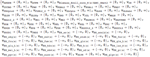
Query all available constraints.
| Out[6]= |  |
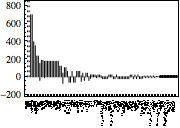
Looking at the flux bounds of all availabe exchange reactions reveals that the current model can only infinitely secrete but not take up any matter.
| Out[15]= |  |
Change a few exchange reaction flux bounds to reflect an aerobic minimal glucose medium.
Flux-balance and flux-variability analysis
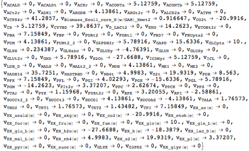
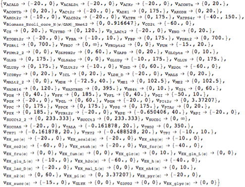
Flux-balance analysis (FBA) finds a steady-state flux solution that maxmizes a cellular objective, e.g., optimal growth rate. For example, FBA can be used to asses the consequence of genetic perturbations. Flux-variablity analysis (FVA) calculates effective flux bounds by minimizing and maximizing flux through individual reactions. For example, FBA solutions are rarely unique and FVA can be used to assess the space of alternativa optimal solutions.
| fba[model, obj] | find a steady-state flux distribution that maximizes obj |
| fva[model] | find minimum and maximum fluxes for all reactions in model |
Basic COBRA functionality
| Out[18]= |  |
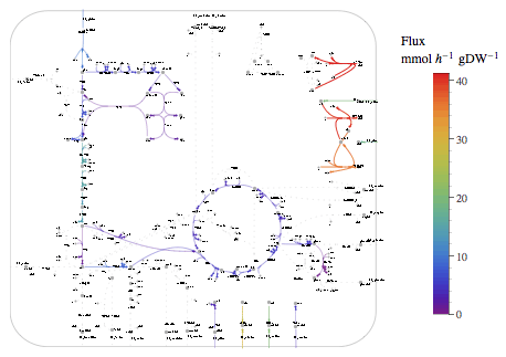
Visualize the fluxes on a pathway map.
| Out[63]= |  |
| Out[24]= |  |
| Out[35]= |  |
High-throughput data integration
| gimme[...] | find a steady-state flux distribution that maximizes obj and matches data |
XXXX.
Changing linear programming solver back-ends
Per default, the toolbox uses
Mathematica's built-in linerar programming solver (
LinerarProgramming). Depending on the availability of other optimization tools, different solver back-ends can be used to solve constraint-based modeling problems.
| LinearProgramming | Mathematica's internal linear programming solver |
| GurobiSolve | MathLink interface to Gurobi |
| GLPKStandalone | Interface to the GLPK standalone solver |
| CPLEXStandalone | Interface to the CPLEX standalone solver |
Supported solver back-ends
Out[60]//Short= |
| |  |
